Radar backscatter derived channel roughness analysis
This is a tutorial of the backscatter for channel roughness analysis using the Google Earth Engine. To get the code, please go to: https://code.earthengine.google.com/024619a64d82577f307f86798bcc1cc3.
Introduction to backscatter analysis
Active and passive remote sensing
Passive sensors:
- The source of radiant energy arises from natural source
- e.g., the sun, Earth, other “hot” bodies
Active sensors:
- Provide their own artificial radiant energy source
- e.g., radar, Synthetic Aperture Radar (SAR), LiDAR
Advantages and disadvantages of radar over optical remote sensing
| Advantages | Disadvantages |
|---|---|
| Nearly all weather capability | Information content is different than optical and sometimes difficult to interpret |
| Day or night capability | Speckle effects (graininess in the image) |
| Penetration through the vegetation canopy | Effect of topography |
| Penetration through the soil | |
| Minimal atmospheric effects | |
| Sensitivity to dielectric properties (liquid vs. frozen water) | |
| Sensitivity to structure |
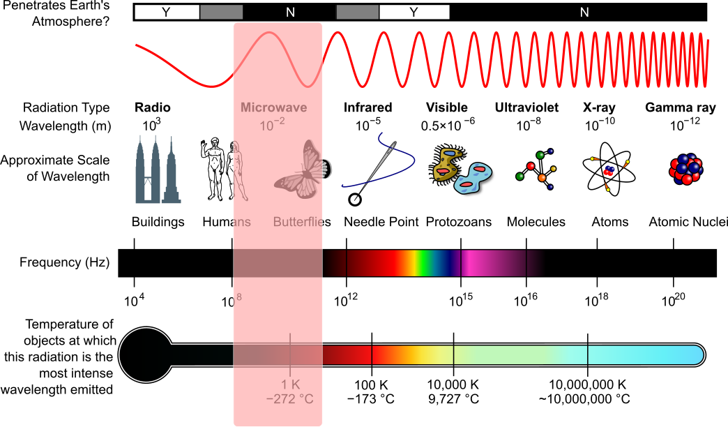
Electromagnetic spectrum
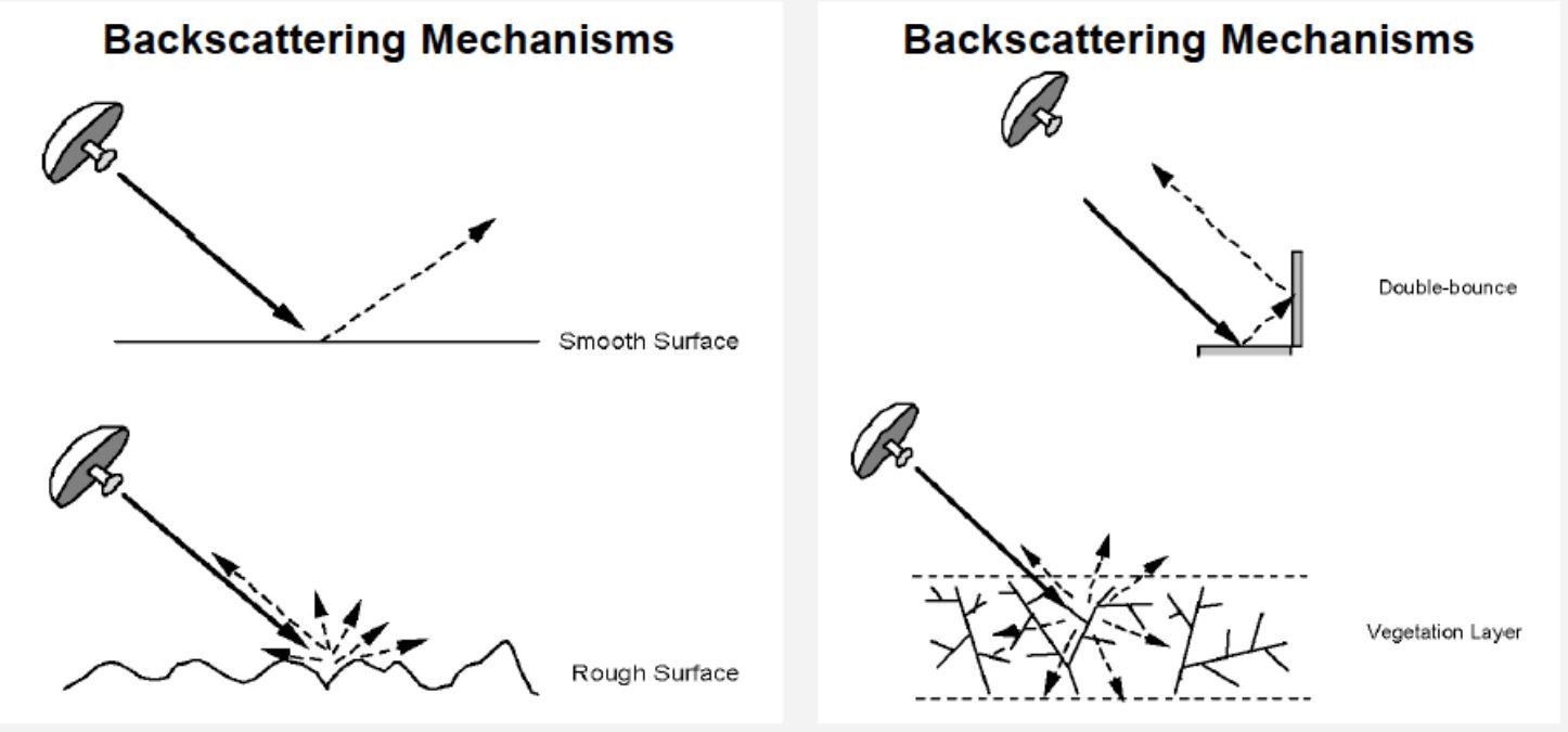
Backscattering mechanism
| Backscatter mechanism | Examples |
|---|---|
| Smooth surface | : e.g., open water, road |
| Rough surface | : e.g., deforested areas, agriculture |
| Vegetation layer | : e.g., Trees canopy |
| Double-bounce | : e.g., inundated area, buildings, structure |
Using GEE for SAR backscatter analysis
First of all, generate an NDVI image which then will be draped above the Satellite image. This is to ensure that the polygons that we use in this analysis do not exceed the channel bank, hence resulting in distorted signal in radar bounce due to vegetation.
var dataset = ee.ImageCollection('LANDSAT/LC08/C01/T1_8DAY_NDVI')
                  .filterDate('2018-01-01', '2020-01-31');
var colorized = dataset.select('NDVI');
print(colorized);
var ndvi=colorized.reduce(ee.Reducer.mean());
print(ndvi);

var ndvi_crop=ndvi.clip(mohand);

var colorizedVis = {
  min: 0.0,
  max: 1.0,
  palette: [
    'FFFFFF', 'CE7E45', 'DF923D', 'F1B555', 'FCD163', '99B718', '74A901',
    '66A000', '529400', '3E8601', '207401', '056201', '004C00', '023B01',
    '012E01', '011D01', '011301'
  ],
};
// Let's centre the map view over the area
Map.centerObject(ROI, 11);
Map.addLayer(ndvi_crop, colorizedVis, 'NDVI');
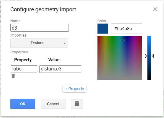
Create series of ‘feature’ rectangles that goes from the outlet of the channel, all the way upstream. Each ‘feature’ properties must be set as:
Import as: Feature Property: Label Value: n (0,1,2,…)
Next, let’s explore and import the Sentinel-1 data. We are going to use the VV polarisation since it demonstrated best response for channel bed roughness analysis (Purinton et al., 2020).
//Filter the collection for the VV product from the Ascending track
var collectionVVas = ee.ImageCollection('COPERNICUS/S1_GRD')
    .filter(ee.Filter.eq('instrumentMode', 'IW'))
    .filter(ee.Filter.listContains('transmitterReceiverPolarisation', 'VV'))
    .filter(ee.Filter.eq('orbitProperties_pass', 'ASCENDING'))
    .filterBounds(mohand)
    .select(['VV']);
print(collectionVVas);
Now let’s show the Sentinel 1 data to the map layer.
var VVas = collectionVVas.median();
Map.addLayer(VVas, {min: -14, max: -1}, 'VVas');
Channel bed analysis works best during the dry season where no water flowing through the channel (that is where the channel bed exposed). In order to do that, we are going to filter our Sentinel-1 data to the desired time frame, the dry season. We are also going to create a ‘3 band stack’ through different dry season periods.
var VV1 = ee.Image(collectionVVas.filterDate('2017-10-30', '2018-05-01').median());
var VV2 = ee.Image(collectionVVas.filterDate('2018-10-30', '2019-05-01').median());
var VV3 = ee.Image(collectionVVas.filterDate('2019-10-30', '2020-05-01').median());
Apply Speckle filtering/smoothing. Smooth the image by convolving with the boxcar kernel.
var boxcar = ee.Kernel.square({radius: 1.5, units: 'pixels', normalize: true});

var VV1n = VV1.convolve(boxcar);
var VV2n = VV2.convolve(boxcar);
var VV3n = VV3.convolve(boxcar);
Create a band stack from different time frame.
var st_vvasc = VV1n.addBands(VV2n).addBands(VV3n);
print('Stacked VV_ASC', st_vvasc);
Map.addLayer(st_vvasc, {min: -12, max: -7}, 'Sentinel-1 Dry Season');
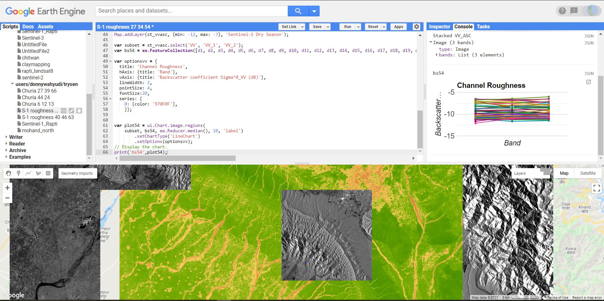
Choose bands to include and define feature collection to use as the backscatter values collection windows.
var subset = st_vvasc.select('VV', 'VV_1', 'VV_2');
var bs54 = ee.FeatureCollection([d1, d2, d3, d4, d5, d6, d7, d8, d9, d10, d11, d12, d13, d14, d15, d16, d17, d18, d19, d20, d21, d22, d23, d24, d25, d26, d28, d29, d30, d31, d32, d33, d34, d35, d36, d37, d38, d39, d40, d41, d42, d43, d44, d45, d46, d47, d48, d49, d50, d51, d52, d53, d54, d55, d56]);
Define the chart to present the radar backscatter values along the channel.
var optionsvv = {
  title: 'Channel Roughness',
  hAxis: {title: 'Band'},
  vAxis: {title: 'Backscatter coefficient Sigma^0_VV (dB)'},
  lineWidth: 2,
  pointSize: 4,
  fontSize:20,
  series: {
    0: {color: '970F0F'},
    }};
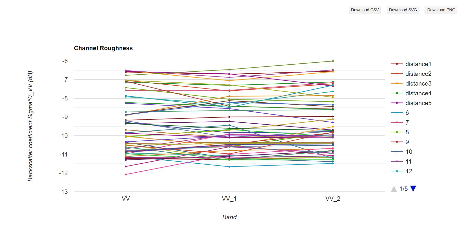
Generate the chart of radar bounce values.
var plot54 = ui.Chart.image.regions(
    subset, bs54, ee.Reducer.median(), 10, 'label')
        .setChartType('LineChart')
        .setOptions(optionsvv);
// Display the chart.
print('bs54',plot54);
Generate the chart to count pixels in every ‘feature’ window.
var plot54c = ui.Chart.image.regions(
    subset, bs54, ee.Reducer.count(), 10, 'label')
        .setChartType('LineChart')
        .setOptions(optionsvv);
// Display the chart.
print('bs54 count',plot54c);
Go to console, and expand the chart by clicking the arrow on the top-right of the chart.
Download the backscatter value as CSV file.
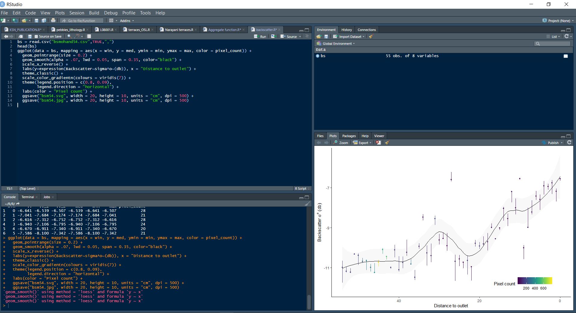
Plot the results in R
bs = read.csv("(your_csv_file).csv",TRUE,",")
head(bs)
ggplot(data = bs, mapping = aes(x = win, y = med, ymin = min, ymax = max, color = pixel_count)) +
  geom_pointrange(size = 0.2) +
  geom_smooth(alpha = .07, lwd = 0.05, span = 0.35, color="black") +
  scale_x_reverse() +
  labs(y=expression(Backscatter~sigma^o~(db)), x = "Distance to outlet") +
  theme_classic() +
  scale_color_gradientn(colours = viridis(7)) +
  theme(legend.position = c(0.8, 0.09),
        legend.direction = "horizontal") +
  labs(color = "Pixel count") +
  ggsave("bsm54.svg", width = 20, height = 10, units = "cm", dpi = 500) +
  ggsave("bsm54.jpg", width = 20, height = 10, units = "cm", dpi = 500)
Here is the result.